COVOID: Age-structured epidemic models in COVOID

Oisin Fitzgerald; Mark Hanly; Tim Churches

Outline

This article introduces the background behind the implementation of age-structured epidemic models in COVOID, in particular:

The rationale behind use the use of age structured epidemic models.
The information needed for the age structured models.
The mathematical model (as a system of ordinary differential equations).
Approaches to modelling the impact of population behaviour changes and/or disease prevention policies.
Calculation of the basic reproduction number and its role in the system dynamics.

Introduction

The transmission and consequences of infection with a virus such as SAR-CoV-2 is influenced by several factors. These include the biology and behaviour of infected individual (host). Both of these components are heavily influenced by (chronological) age. People spend a disproportionately large amount of their time in particular settings such kindergartens, school, workplaces and households.¹ This skews their chance of contacting certain age groups. Accounting for non-uniform age contacts in compartmental epidemic models can aid in understanding the potential impact and dynamics of disease in a population. Further, it enables more realistic modelling of disease prevention policy.

For example, on average individuals over 60 years have four less contacts with others per day compared to the societal average.¹ Lower contact rates reduces their number of opportunities to spread or contract a virus. Age is also associated with susceptibility to viral infection, children have been shown to be more susceptible to influenza compared to adults.² Considering COVID-19, increased age is associated with higher mortality rates, with evidence of a fivefold increase in risk of death for individuals aged over 60 years compared to under 60 years.³ COVOID is motivated by the need to incorporate available data on population structure and the impact of interventions, while building upon ordinary differential equation (ODE) based compartmental epidemic models to enable rapid turnaround in disease modelling.

ODE based compartmental models (e.g. the SIR model) are a key tool of mathematical epidemiology that involve modelling the flow of move of individuals from non-disease through (possibly many) disease states. These model can be seen as a (mean-field) approximation to an underlying stochastic process, providing us with estimates of the “average outcome.”⁴ They have traditionally been used assuming homogeneous mixing of the population. The distribution of contact rates for individuals can be well described by a single (empirical) average contact rate. If we consider any partition of the population into $j=1,...J$ groups (e.g. based on age, gender, pre-existing illness) the homogeneous case assumes a contact rate and infection probability between individuals in group i and j of $c_{ij} = c$ and $\beta_{ij} = \beta$. Homogeneous models have several advantages; they enable easy programming and estimation of parameters, and have well studied behaviours (e.g. the relationship between parameters such as the basic reproduction number $\mathcal{R_0}$ and epidemic size). However, through modelling the distribution of contact rates as a single they make it difficult to separate the impact of various interventions and behaviours.

For example, it is difficult to model how school closure differs from physical distancing, or variation in transmissibility across age groups.⁵ Further, they limit incorporation of available detailed epidemiological or demographic data. Studies such as 6 and 7 provide detailed info about age specific contacts and many health authorities provide age specific incidence rates on current epidemics (e.g. NSW Health). This allows for data-driven increases in the realism of these models. We move to a case where $c_{ij}$ or $\beta_{ij}$ vary depending on group $i$ and $j$. These models are more complex and exhibit different system dynamics e.g. $\mathcal{R_0}$ no longer a simple ratio as in homogeneous model. This is something that is important to consider and sensitivity analysis plays an important role in complex DCMs. Further, these models are still producing averages, which provide a poor description of heavy-tailed distributions arguably important in epidemics due, for example, to super-spreader events.⁸

Looking ahead, this article describes the basics of the theoretical background and other considerations when moving from the homogeneous compartmental model to more complex (discrete) age structured models, and the basics of how to use COVOID to model these situations (for more on the programming API see vignette('age-structure-mixing')). We firstly describe what information is needed, the mathematical model for an SIR example and the general SEIR case and calculation of the basic reproduction number. Throughout we will assume stable demography, i.e. no migration and birth or death. This assumption is reasonable over short time frames where the distribution of individuals is unlikely to shift sufficiently to result in large groups of newly uninfected individuals. However it should be relaxed for longer time frames.

Age structured population

In order to introduce heterogeneity in the average population contact rates we may require a great deal more information. A basic homogeneous compartmental model requires estimates of the population size $N$, broken down into the given compartments (e.g. $S$, $I$ and $R$), along with disease dynamics parameters. At the very least these includes two of $\beta$, the probability of infection given contact, $c$, the contact rate and $\gamma$, the inverse of the length of illness. Two key addition for the varying the contact rate by group are the contact rates between the different groups and distributions of these groups in the population. For $J$ groups this an additional $J(J + 1)$ parameters. Thankfully, previous researchers and organisations have made age distributions and age-specific contact matrices split into different settings such as home, school, work and other.^6,9

Previous research by 6 has created contact matrices for five year age groups for 152 countries, see figure 1. COVOID builds upon this research to allow the modelling of a particular population as being composed of $i = 1,...,16$ discrete age groups (e.g. (0,5], (5,10],…(75,80]. Each element $c_{ij}$ of a contact matrix is the average contact rate between individuals in group $i$ with individuals in group $j$. Within COVOID these matrices can be imported for ~150 countries - see available_contact_matrices() for the full list - using the import_contact_matrix function which takes the arguments country and setting. The setting can be one of “school”, “work”, “other”, “home” or “general”. The general matrix is the sum of the other four. A plot method utilising ggplot2 has been introduced for these matrices allowing quick visualising (see figure 1).

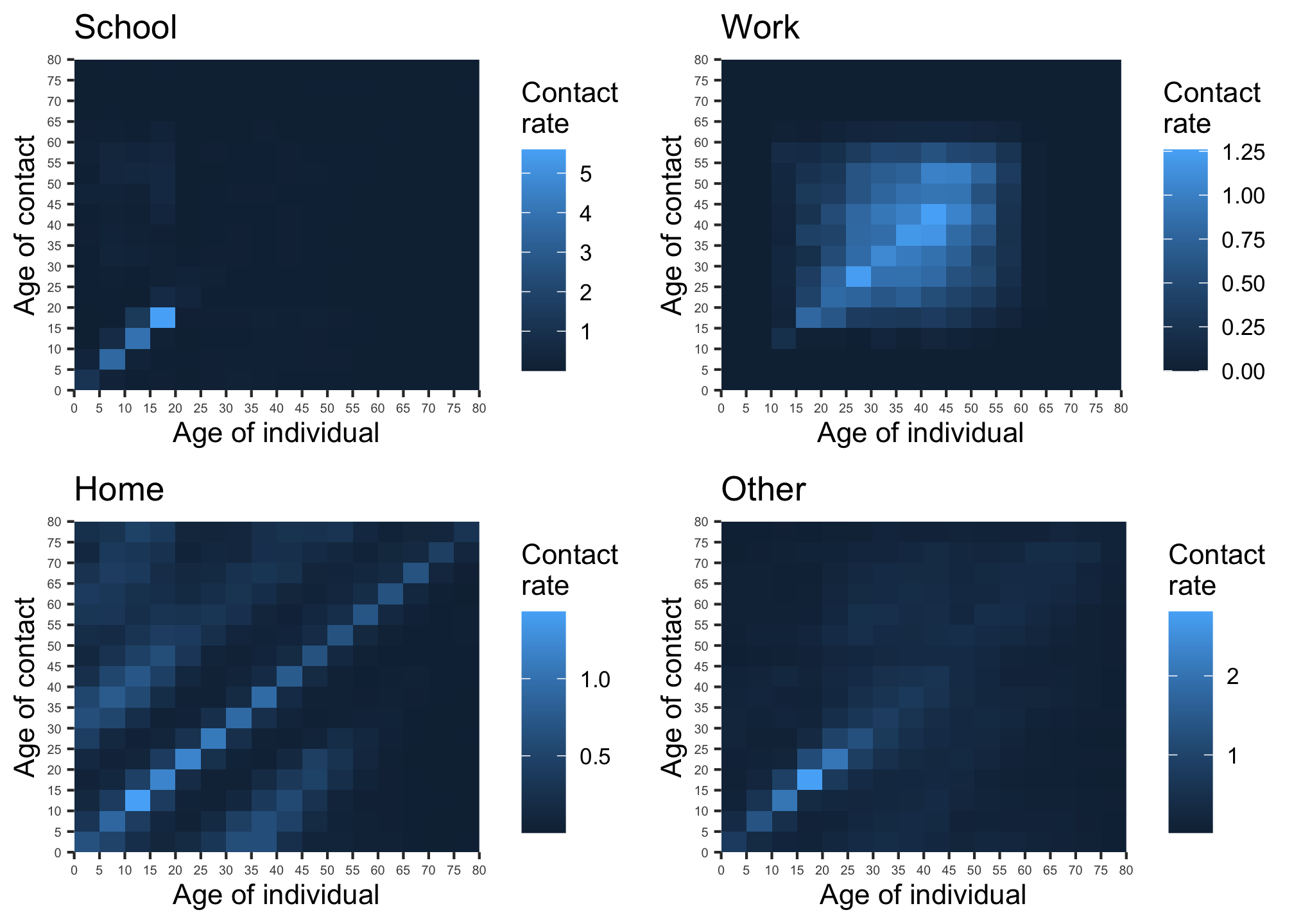
Contact matrices for school, work, home and other locations (source: @prem2017projecting). Note the differing scales.

Figure 1: Contact matrices for school, work, home and other locations (source: 6). Note the differing scales.

The COVOID package also contains age distributions for ~150 countries, original compiled by 9. These are proportions $p_i$ in each age category from (0,5], (5,10],…,(75,80]. These can be imported imported using import_age_distribution function. - see age_distributions_un() for the full list of available countries. A plot method utilising ggplot2 has been introduced for these allowing quick visualising (see figure 2).

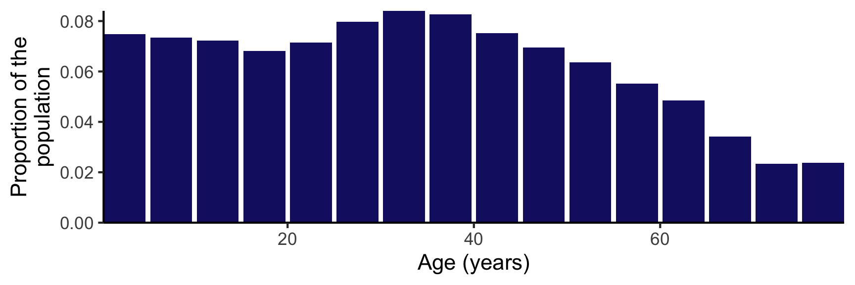
Figure 2: Age distribution of the Australian population

We note that the contact matrices are not symmetric. The contact rate between an individual in age group $i$ and age group $j$ is $c_{ij}$. Generally $c_{ij} \ne c_{ji}$ due to the non-uniform distribution of age in human societies. The lack of symmetry is illustrated in figure 1. However, it should be the case that $p_ic_{ij} = p_jc_{ji}$. The number of contacts of group $i$ with group $j$ should equal the number of contact by group $j$ with group $i$ (see note A).

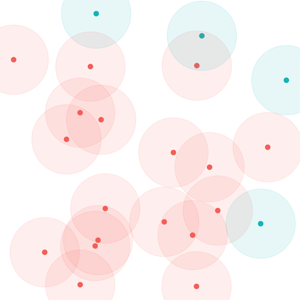
Asymmetry of contact rates due to non-uniform distribution into partitions (red/blue). Each point represents an individual and the shaded area the individuals they will contact in the next time step. On average each red will contact ~2 reds, and ~0.2 blues. Blues will meet ~0.8 red and 0 blues.

Figure 3: Asymmetry of contact rates due to non-uniform distribution into partitions (red/blue). Each point represents an individual and the shaded area the individuals they will contact in the next time step. On average each red will contact ~2 reds, and ~0.2 blues. Blues will meet ~0.8 red and 0 blues.

General mathematical model

Figure 4: SEIR model forward dynamics

Extending the SIR/SEIR models to account for heterogeneous mixing across a discrete structure such as age groups is largely an exercise in indexing the system dynamics. In the next section we will introduce the approach for interventions. There are $N_j$ individuals in each of the $j = 1,...,J$ age groups, with susceptible-exposed-infected-removed compartments $S_j$, $E_j$, $I_j$ and $R_j$. The proportion of the population in a particular age group is $p_j = \frac{N_j}{N}$.

Taking the viewpoint of a susceptible individual in an arbitrary age group $S_j$, this individual meets $c_{jk}$ individuals in age group $k$ per day. Of these the proportion that are infected is $\frac{I_k}{N_k}$. Assume a constant probability of disease transmission $\beta$. Combining these terms we have the chance a susceptible individual in $S_j$ meets and is infected by an individual in $I_k$ is $\beta c_{jk} \frac{I_k}{N_k}$. Summing this over all susceptible individuals in $j$, and all infected in k$ gives us time rate of change in $S_j$ due to infections of

\[ \begin{align} \frac{dS_j}{dt} &= -\sum_{j=1}^{|S_j|} \sum_{k=1}^{K} \beta c_{jk} \frac{I_k}{N_k} \\ \frac{dS_j}{dt} &= -S_j \sum_{k=1}^{K} \beta c_{jk} \frac{I_k}{N_k} \\ \end{align} \] For infections such as COVID-19 it has become common practise to split the E/I compartments in further subsections, to account for the pattern in which the infectiousness and symptomatic phases overlap, and wide variation in severity. If we denote these $L = L_E + L_I$ disease periods for age group $k$ as $E_{kl}$ and $I_{kl}$, with infectiousness present from stage $I_{k1}$ the above extends to

\[ \begin{align} \frac{dS_j}{dt} &= -S_j \sum_{k=1}^{K} \beta c_{jk} \sum_{l=1}^{L_E} \frac{I_{kl}}{N_k} \\ \end{align} \] The remainder of the disease dynamics is relatively straightforward, letting the average amount of time spent in $E_{*l}$ be $\sigma_l$ and $I_{*l}$ to be $\gamma_l$ we have a system of the form

\[ \begin{align} \frac{dS_j}{dt} &= -S_j \sum_{k=1}^{K} \beta c_{jk} \sum_{l=1}^{L_E} \frac{I_{kl}}{N_k} \\ \frac{dE_{j1}}{dt} &= S_j \sum_{k=1}^{K} \beta c_{jk} \sum_{l=1}^{L_E} \frac{I_{kl}}{N_k} - \sigma_1 E_{j1} \\ ... \\ \frac{dI_{j1}}{dt} &= \sigma_{L_E} I_{jL_E} - \gamma_{1} I_{j1}\\ ... \\ \frac{dR_{j}}{dt} &= \gamma_{L_I} I_{jL_I} \\ ... \\ \end{align} \]

In COVOID these models are solved using the deSolve::ode function from the R package deSolve which uses numerical integration methods such as the Runge-Kutta algorithms.¹⁰

An example: two age groups

This example is aimed at illustrating how the introduction of contact matrices influences the behaviour of the system. Consider a population with two age groups - adults and children. Our contact matrix in table 1 shows that a child has on average 5.8 contacts per day with other children and 2.6 contacts with an adult. The proportion of adults and children in the population is $p_a = \frac{2}{3}$ and $p_c = \frac{1}{3}$, with the subscripts $a$ and $c$ denoting adult and child. Notice that $p_a c_{ac} = p_c c_{ca}$ as expected.

Table 1: COntact rates between adults and children. Source: 11
	Individual: child	Individual: adult
Contact: child	5.8	1.3
Contact: adult	2.6	1.9

Our SIR system, dropping $\frac{dR_i}{dt}$ as it is not relevant to the spread of the infection, is

\[ \begin{align} \frac{dS_c}{dt} &= -S_c\beta(c_{cc}\frac{I_c}{N_c} + c_{ca}\frac{I_a}{N_a}) \\ \frac{dS_a}{dt} &= -S_a\beta(c_{aa}\frac{I_a}{N_a} + c_{ac}\frac{I_c}{N_c}) \\ \frac{dI_c}{dt} &= S_a\beta(c_{aa}\frac{I_a}{N_a} + c_{ac}\frac{I_c}{N_c}) - \gamma I_c\\ \frac{dI_a}{dt} &= S_a\beta(c_{aa}\frac{I_a}{N_a} + c_{ac}\frac{I_c}{N_c}) - \gamma I_a\\ \end{align} \]

An initial run of the model, with with $\beta = 0.1$, $\gamma = 0.2$ and a population size of $N=10,000$. We see the epidemic peaks around $t=50$ and ultimately infects about 80% of the population. Note the difference between adults and children in this example. Now, the initial conditions and contact matrices can alter the timing and evolution of the epidemic.

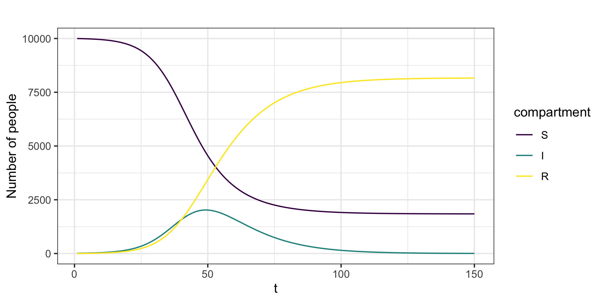
Figure 5: Example epidemic trajectory

For example, if we maintain a starting cohort of 11 infectives put vary the proportion in each group we can shift the timing of the epidemic peak. As shown by figure 6 there is a 25 unit shift between the case where the infection begins in the children or adult group.

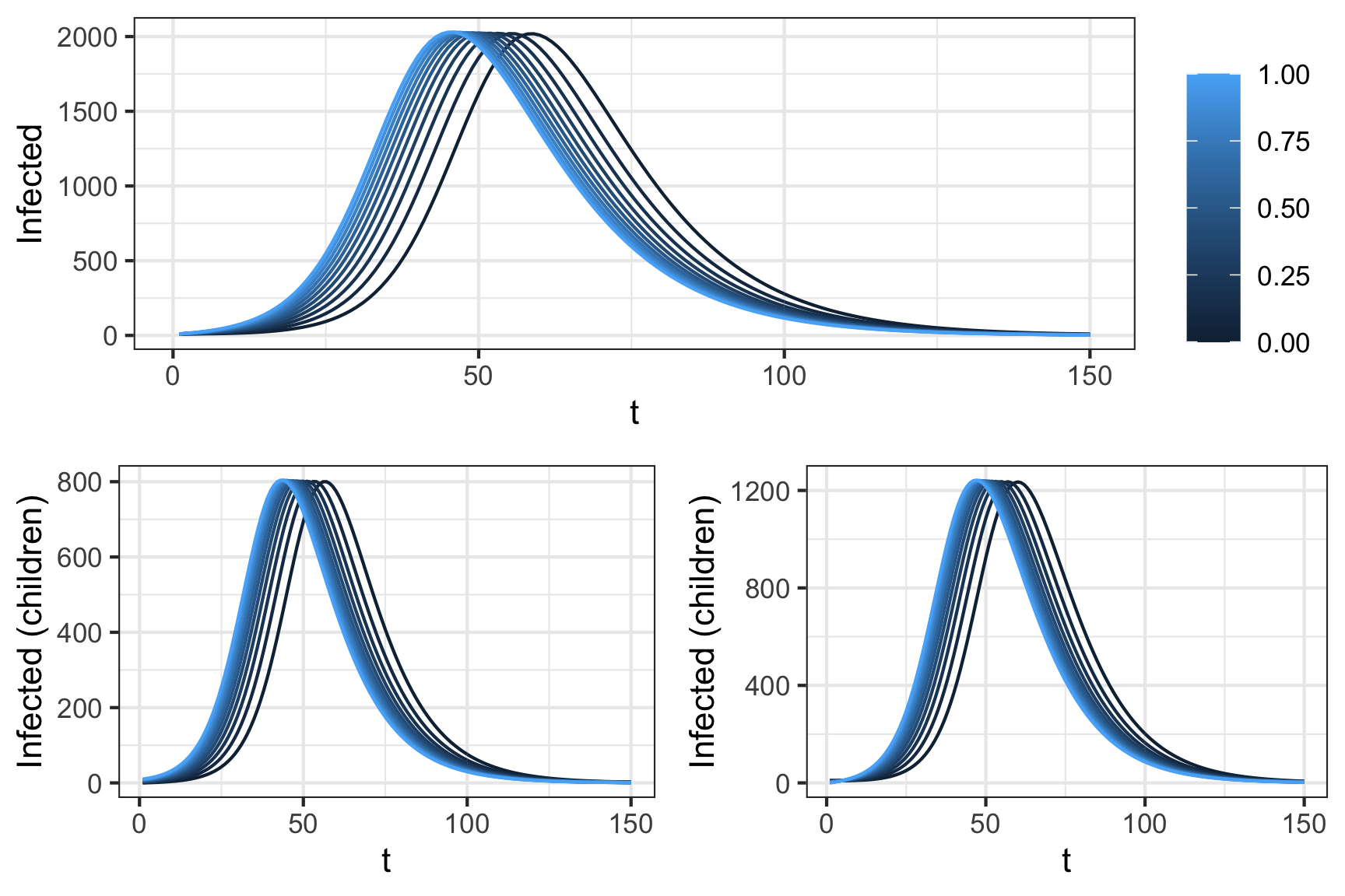
Figure 6: Impact of initial conditions on disease peak. All simulations atart with 10 infected individuals, dispersed over

To further illustrate the impact of the contact matrix notice what happens when we alter the contact matrix to reduce inter-group contact while maintaining the same overall levels of contact. In this case we vary the $\alpha$ parameter in the table below from 0 to 1. At $\alpha = 0$ we isolate each group from one another. The number initially infected are 10 in each group. Notice that for $\alpha = 0$ the infection never takes hold in the adults. Indeed the value of $\mathcal{R_0}$ in the isolated adults group is 0.5. This case reflects an intuition that epidemics are driven by those with large numbers of contacts (although we are strictly considering average here). For more on this topic see 12.

Table 2: Varying the contact rate, the $\alpha$ parameter varies from 0 to 1. Source: 11
	Individual: child	Individual: adult
Contact: child	5.8 + ($1-\alpha$) 2.6	$\alpha$ 1.3
Contact: adult	$\alpha$ 2.6	1.9 + ($1-\alpha$) 1.3

Figure 7: Final epidemic size and initial contact matrix

Clearly even in this simple case the initial conditions and variation in the contact matrix alter the predicted evolution of the epidemic, illustrating the importance of careful consideration and thought in how these models are structured and the need for sensitivity analysis. The choice of contact matrix, and distributions across compartments influence the final epidemic size and timing.

Modelling interventions

Interventions (e.g. social distancing) can reduce either the contact rate $c_{ij}$ or the probability of transmission $\beta$. As these terms are linearly combined in the SIR/SEIR models we don’t differentiate our interventions act upon one or both. An intervention that reduces the tranmissibility $\beta c_{ij} = \tau_{ij}$ of the disease from group $i$ to $j$ is denoted by $Y_{ij}(t)$ and takes a value in $(0,1)$. Some interventions may act at certain stages, for example self-isolation of people with respiratory symptoms, leading to a general form

\[\frac{dS}{dt} = - S_i \sum_{j=1}^{J} \tau_{ij} \sum_{k=1}^{K} Y_{kij} \frac{I_{kj}}{N_j}\]

COVOID allows $Y_{kij}(t)$ to be a smooth function - e.g. logistic function or a step function. This allow for cases where an intervention takes effect immediately (e.g. no flights) or gradually (e.g. voluntary physical distancing).

The basic reproduction number

The basic reproduction number $\mathcal{R_0}$ is defined as the average number of secondary infections arising from a single individual during their entire infectious period, in a population of susceptibles.¹³ In many models (including those under discussion) $\mathcal{R_0}$ is related to the peak and final spread of a epidemic, and acts as a threshold parameter for invasion of a disease organism into a completely susceptible population.¹⁴ However, for complex models there is not a uniformly accepted method for calculating $\mathcal{R_0}$. As shown by 15 the various methods give different answers. With this qualification we describe the next generation approach to calculation of $\mathcal{R_0}$. This approach is used by in COVOID package and other authors^16,17 to calculate $\mathcal{R_0}$ and/or translate $\mathcal{R_0}$ into more basic quantities.

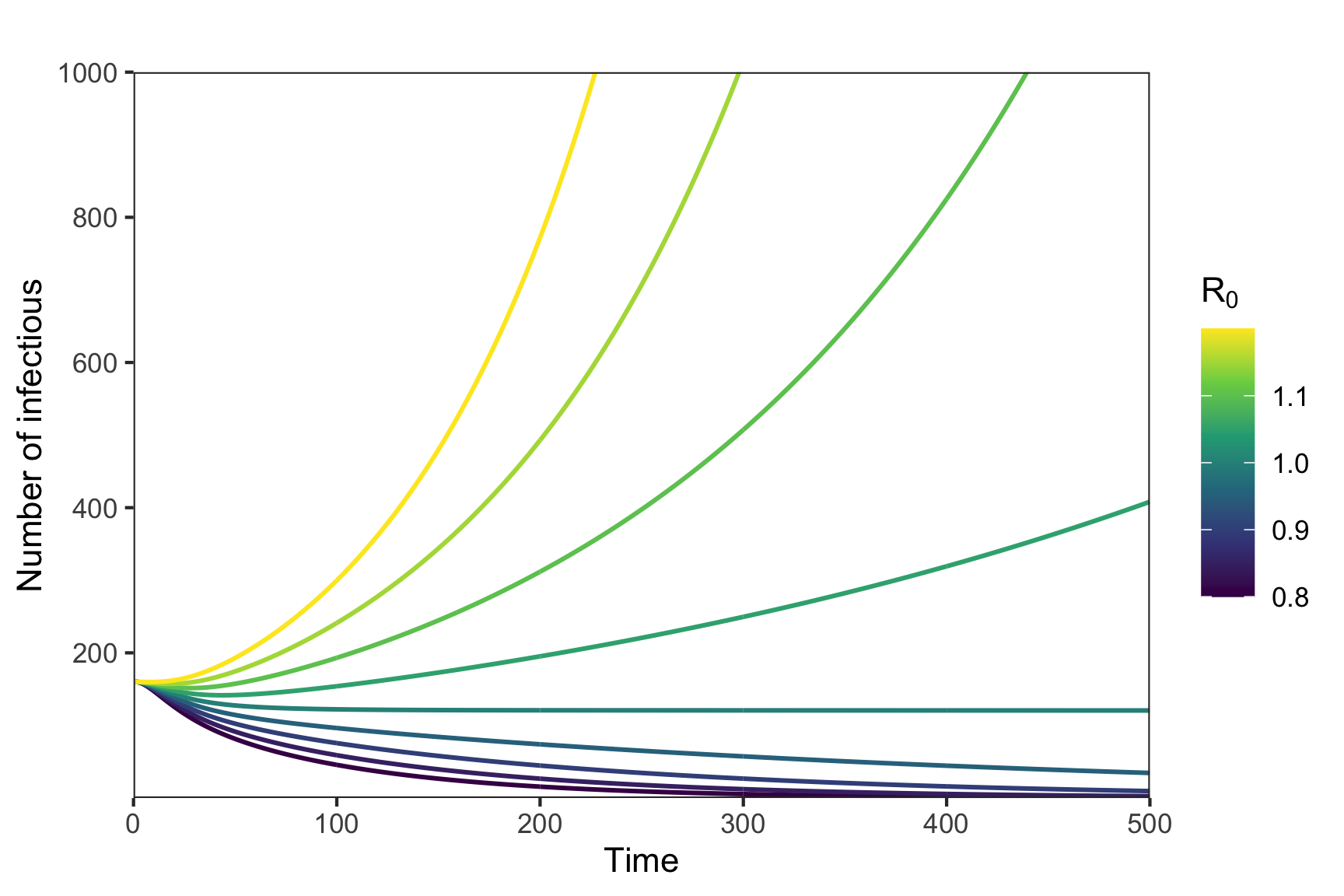
Figure 8: Potential for exponential growth and $R_0$

We will consider the generalised SEIR case, in which $E_j$ and $I_j$ compartments may be further decomposed into $E_{j1},...,E_{jn_1}$ and $I_{j1},...,I_{jn_2}$. Changing nomenclature a little, let $y \in \mathbb{R}^m$ be m-vector of non-disease compartments and $x \in \mathbb{R}^n$ the n-vector of disease compartments. For example $y = (S_1$,…,$S_J)$ and $y = (E_{11}$,…,$I_{Jn_2})$. Note that we can ignore R for the case of no reinfection as it simply acts as an end-state reservoir. The time derivative of $x$ is $x_i' =\mathcal{F_i}(x) - \mathcal{V_i}(x)$, where $\mathcal{F}(x)$ is the rate secondary infections increase the $i^{th}$ compartment and $\mathcal{V}$ is the rate of disease progression out of the $i^{th}$ compartment. We then construct the matrices $F$ with elements $\frac{\partial \mathcal{F_i}}{\partial x_i}(x_0)$ and $V$ with elements $\frac{\partial \mathcal{V_i}}{\partial x_i}(x_0)$. The state vector $x_0$ is a vector of zeros referred to as the disease free equilibrium, the point at which no disease is present in the population.¹⁸ The next generation matrix is $K = FV^{-1}$. It can be understood as a linearisation of the non-linear SIR system over a short time period near the disease free equilibrium. The basic reproduction number is can be calculated from it as $\mathcal{R_0} = \rho(K)$ where $\rho(K)$ is the spectral radius or maximum of the absolute values of the eigenvalues of $K$. For example, using the contact matrix and population distribution information from an SIR model with two population groups we have

\[ \begin{align} \mathcal{F_1} &= S_1(\beta c_{11} \frac{I_1}{N_1} + \beta c_{12} \frac{I_2}{N_2}) \\ \mathcal{F_2} &= S_2(\beta c_{21} \frac{I_1}{N_1} + \beta c_{22} \frac{I_2}{N_2}) \\ \\ F &= \begin{pmatrix} \frac{\partial \mathcal{F_1}}{\partial I_1} & \frac{\partial \mathcal{F_2}}{\partial I_1} \\ \frac{\partial \mathcal{F_1}}{\partial I_2} & \frac{\partial \mathcal{F_2}}{\partial I_2} \\ \end{pmatrix} \\ &= \begin{pmatrix} \beta c_{12} & \frac{p_1}{p_2} \beta c_{12} \\ \frac{p_2}{p_1} \beta c_{21} & \beta c_{22} \\ \end{pmatrix} \end{align} \]

Where we remind the reader that $p_j = \frac{N_j}{N}$, and $S_j = N_j$ since we in the state of disease free equilibrium. Since $\mathcal{V} = \gamma I_j$ its derivative with respect to $I_j$ is just $\gamma$ giving $V = \gamma I_n$, where $I_n$ is an $n \times n$ identity matrix, and $V^{-1} = \frac{1}{\gamma} I_n$. Multiplying $F$ and $V^{-1}$ gives

\[ \begin{align} K &= \frac{1}{\gamma}\begin{pmatrix} \beta c_{12} & \frac{p_1}{p_2} \beta c_{12} \\ \frac{p_2}{p_1} \beta c_{21} & \beta c_{22} \\ \end{pmatrix} \\ \end{align} \]

Solving for $det(K-\lambda I)$ (using 19) gives a characteristic equation with solutions $\lambda_{\pm} = \frac{1}{2}[\frac{\beta}{\gamma}(c_{11} + c_{22}) \pm \beta \sqrt{4f_1f_2\frac{1}{\gamma}c_{12}c_{21} + \frac{1}{\gamma^2} (c_{11}^2 + c_{22}^2 - 2 c_{11} c_{22} )}]$, where $f_1 = \frac{p_1}{p_2}$ and $f_2 = \frac{p_2}{p_1}$. While an unwieldy equation, we show it here for two reasons, firstly simply to point out that if $f_1 = f_2$ and $c_{ij} = c_{ji}$ for all $i,j$ pairs then it reduces to the familiar $\frac{\beta c}{\gamma}$ for the homogeneous SIR model. Secondly, plotting the value of $\mathcal{R_0}$ for various values of $c_{ij}$ and $f_j$ can illustrate properties of the system (as per the adult-child structured example). More practically for a general $F$ and $V$ can also numerically solve for $\mathcal{R_0}$, e.g. using the following R script:


# parameters
gamma <- 0.2
beta <- 0.1
cm <- matrix(c(5.8,1.3,2.6,1.9),ncol=2,byrow = TRUE)
dist <- c(1/3,2/3)
# calculate next generation matrix
V <- diag(rep(gamma,2))
F1 <- cm
for (i in 1:2) {
  for (j in 1:2) {
    F1[i,j] <- (dist[i]/dist[j])*beta*F1[i,j]
  }
}
FF <- F1
# K is the next generation matrix
K <- FF %*% solve(V)
ee <- eigen(K)
R0 <- max(abs(Re(ee$values)))
cat("R0:",R0)
#> R0: 3.265009

Conclusion

We have outlined the some of the background behind the COVOID package and app. The mathematics of extending a homogeneous SIR/SEIR model to account for greater heterogeneity in the population via contact matrices and age distributions are straightforward. However, the behaviour of the system is much more complex, emphasising the need for sensitivity analysis and clarity around assumptions. Nevertheless these models are a powerful approach to modelling differing forms of interventions and situations in which assumptions of equal contact and infectiousness or susceptibility across a population are not valid.

Notes

A: Contact matrices
As COVOID sources the contact matrices and age distributions from different sources this equality is unlikely to hold exactly for all cases. The error can be checked by constructing a matrix of elements $M_{ij} = p_ic_{ij}$ and examining $M - M^t$ where $t$ denotes the transpose. Care should be taken to examine the impact of any error, including any difference in results in cases of certain symmetry (e.g. using $\frac{1}{2}(M + M^t)$).

Age-structured epidemic models in COVOID

Outline

Introduction

Age structured population

General mathematical model

An example: two age groups

Modelling interventions

The basic reproduction number

Conclusion

Notes

Further reading

Corrections

Reuse

Citation

	Individual: child	Individual: adult
Contact: child	5.8 + (\(1-\alpha\)) 2.6	\(\alpha\) 1.3
Contact: adult	\(\alpha\) 2.6	1.9 + (\(1-\alpha\)) 1.3