Outline
This vignette introduces the COVOID programming API for modelling age-structured epidemic models in COVOID. It covers:
- The use of contact matrices.
- Modelling interventions/behaviour changes that reduce contact rates in different settings
- Modelling variation in infectiousness/susceptibility
Base case - no interventions/behaviour changes
For our examples we’ll consider an epidemic in a population of 5 million, modelled on the population of Sydney, Australia. We can import contact matrices and age distributions for ~150 countries and plot these using plot methods.
# import contact matrix and age distribution
cm_oz <- import_contact_matrix("Australia","general")
p_age_oz <- import_age_distribution("Australia")
# use covoid plotting methods
plot(cm_oz)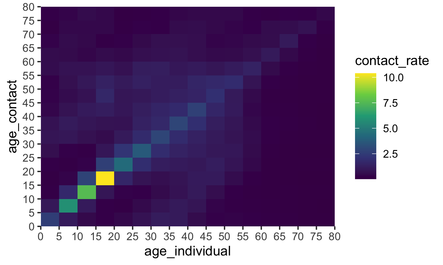
plot(p_age_oz)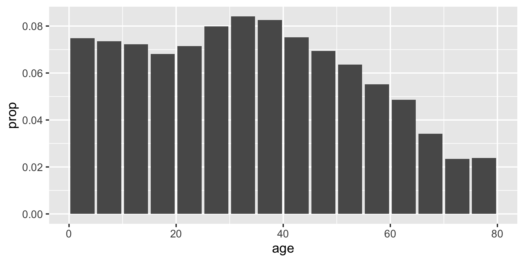
These plots are ggplot objects (i.e. class(plot(p_age_oz)) gives gg, ggplot) allowing further customisation beyond the basic default appearance.
We’ll start the epidemic simulation with ~50 cases, distributed geometrically between the ages of 20 and 80, roughly matching age distribution and early March incidence information available from NSW Health.
# initial conditions
S <- p_age_oz*5e6
E <- c(0,0,0,0,ceiling(7*(0.9)^(1:12)))
I <- rep(0,length(S))
R <- rep(0,length(S))
We first consider the case without any intervention, letting the epidemic run its course. The epidemic peaks ~220 days after time zero, with an . If we are using a model with the code * we pass the parameters for the ODE system to the *_param function, the initial compartment states to *_state0 and finally run the system using simulate_*. A plot method (built using ggplot2) for the resulting object of class covoid allows quick visualisation of the evolution of the compartments over time.
param <- seir_c_param(R0 = 2.5,gamma = 0.1,sigma=0.1,cm=cm_oz,dist=p_age_oz)
state0 <- seir_c_state0(S = S,E = E,I = I,R = R)
res <- simulate_seir_c(t = 500,state_t0 = state0,param = param)
plot(res,y=c("S","E","I","R"),main="No intervention")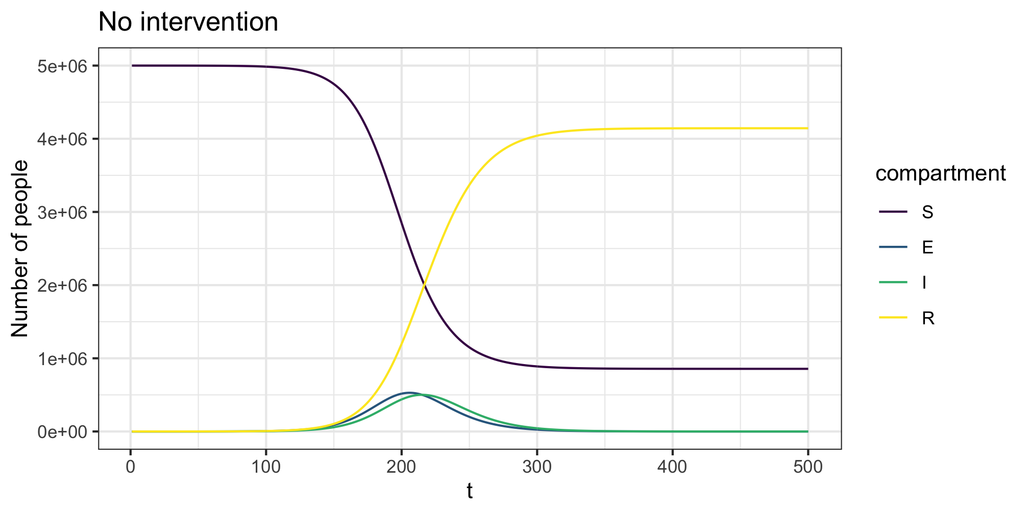
Interventions and behaviour change
We can add in time varying changes in person to person contact rates using the contact_intervention function. This function allows specification of the start and stop times of the intervention, along with potential delays until full adoption. These “interventions” are not only government mandated behaviour changes but any shift in individual behaviour that could reasonably be expected to alter the levels of person-person physical interaction in the population under study. The below example reduces all contact by 20%. This could be considered to be simulating mild physical distancing. Note the ~50 day right shift in the epidemic trajectory. As we end the physical distancing before complete suppression it still has the same outcome.
# interventions
phys_dist <- contact_intervention(start = 10,stop = 150,reduce = 0.8,
                                 start_delay = 5,stop_delay = 5)
# model and simulation
param <- seir_c_param(R0 = 2.5,gamma = 0.1,sigma=0.1,cm=cm_oz,dist=p_age_oz,
                     contact_intervention = phys_dist)
state0 <- seir_c_state0(S = S,E = E,I = I,R = R)
res <- simulate_seir_c(t = 500,state_t0 = state0,param = param)
plot(res,y=c("S","E","I","R"),main="Physical distancing")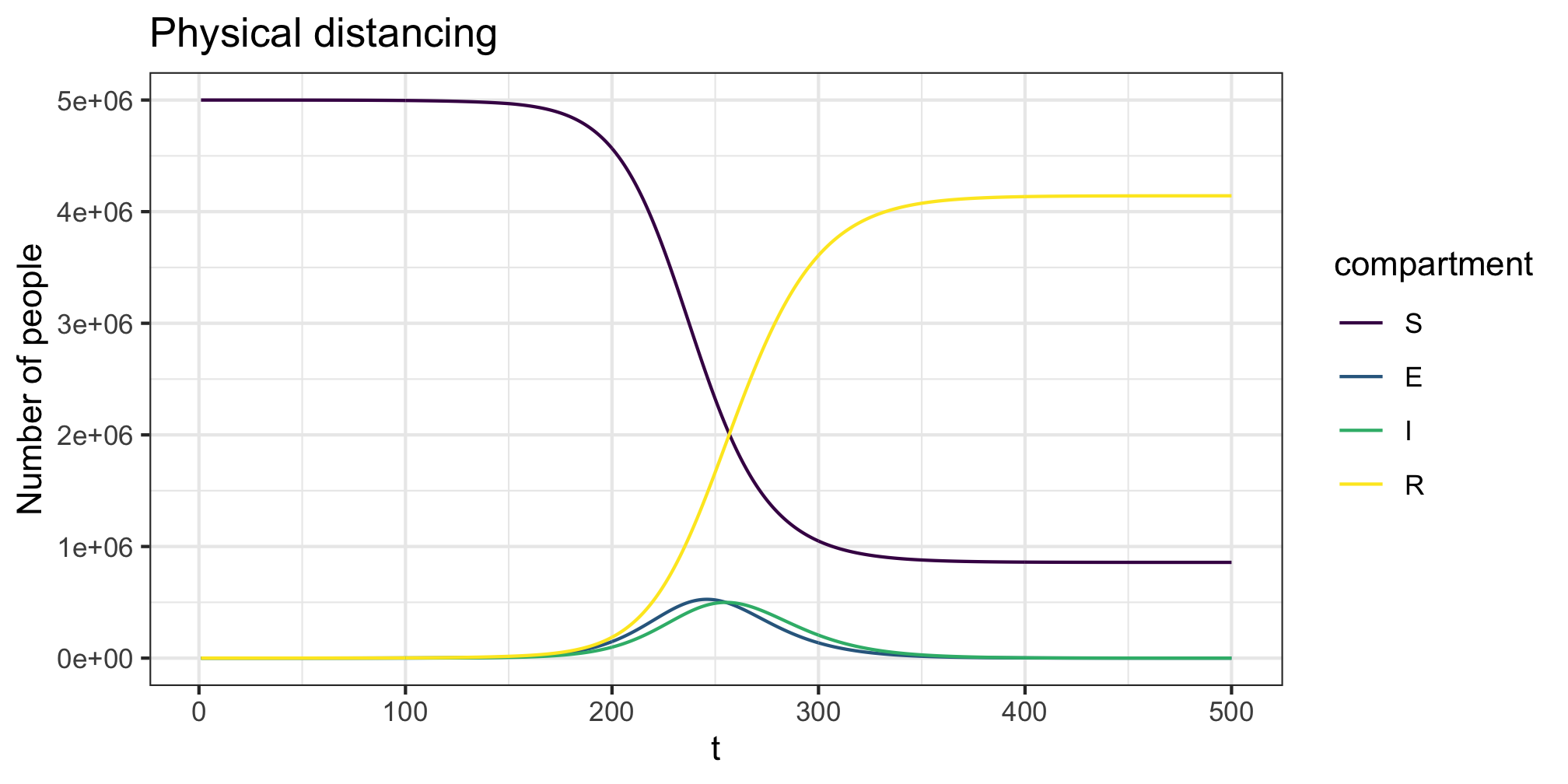
The COVOID package allows you to separate the contact rates into different settings - e.g. school, work and home. For example, using the “general” and “school” contact matrices for Australia we have the below patterns of interaction.
cm_oz_all <- import_contact_matrix("Australia","general")
cm_oz_sch <- import_contact_matrix("Australia","school")
# separate out school and general population contact rates
cm_oz_all <- cm_oz_all - cm_oz_sch
p_all <- plot(cm_oz_all) + labs(title = "General") +
  theme(axis.text.x = element_text(size=6, angle=0),
          axis.text.y = element_text(size=6))
p_sch <- plot(cm_oz_sch) + labs(title = "School") +
  theme(axis.text.x = element_text(size=6, angle=0),
          axis.text.y = element_text(size=6))
gridExtra::grid.arrange(p_all,p_sch,ncol=2)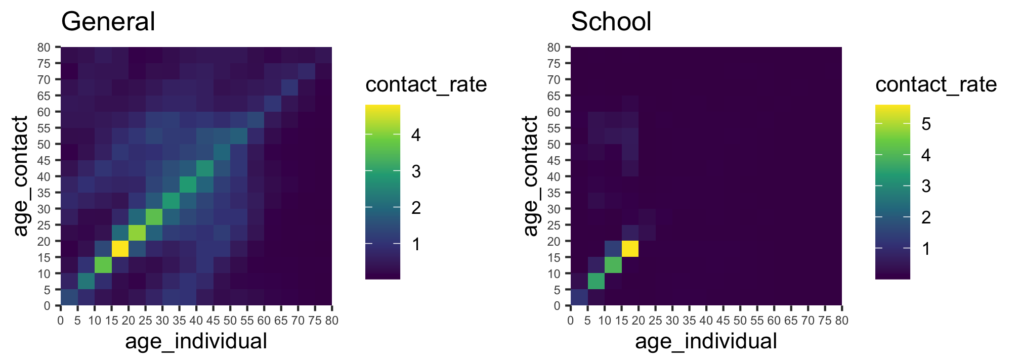
We can then add in time varying interventions using create_intervention to each setting. We do this by creating two list objects, one for the contact matrices and the other for the interventions. Each list must be named with the setting names matching across the contact matrix and intervention lists. For example, all and sch in the example below. For this example we again reduce general contact rates in the population by 20% to simulate physical distancing and combine it with a reduction in school age contact by 80% to simulate school closures. Again we see a slight ~25 day right shift in the epidemic trajectory with early ending of interventions leading to a similar final outcome to the no behaviour change setting.
# contact matrices and interventions
cm <- list(all = cm_oz_all, sch = cm_oz_sch)
int <- list(sch=contact_intervention(start = 10,stop = 150,reduce = 0.2,
                                    start_delay = 5,stop_delay = 5),
           all=contact_intervention(start = 10,stop = 150,reduce = 0.8,
                                    start_delay = 5,stop_delay = 5))
# model and simulation
param <- seir_c_param(R0 = 2.5,gamma = 0.1,sigma=0.1,cm=cm,
                      dist=p_age_oz,contact_intervention = int)
state0 <- seir_c_state0(S = S,E =E,I = I,R = R)
res <- simulate_seir_c(t = 500,state_t0 = state0,param = param)
plot(res,y=c("S","E","I","R"),main="Physical distancing and school closures")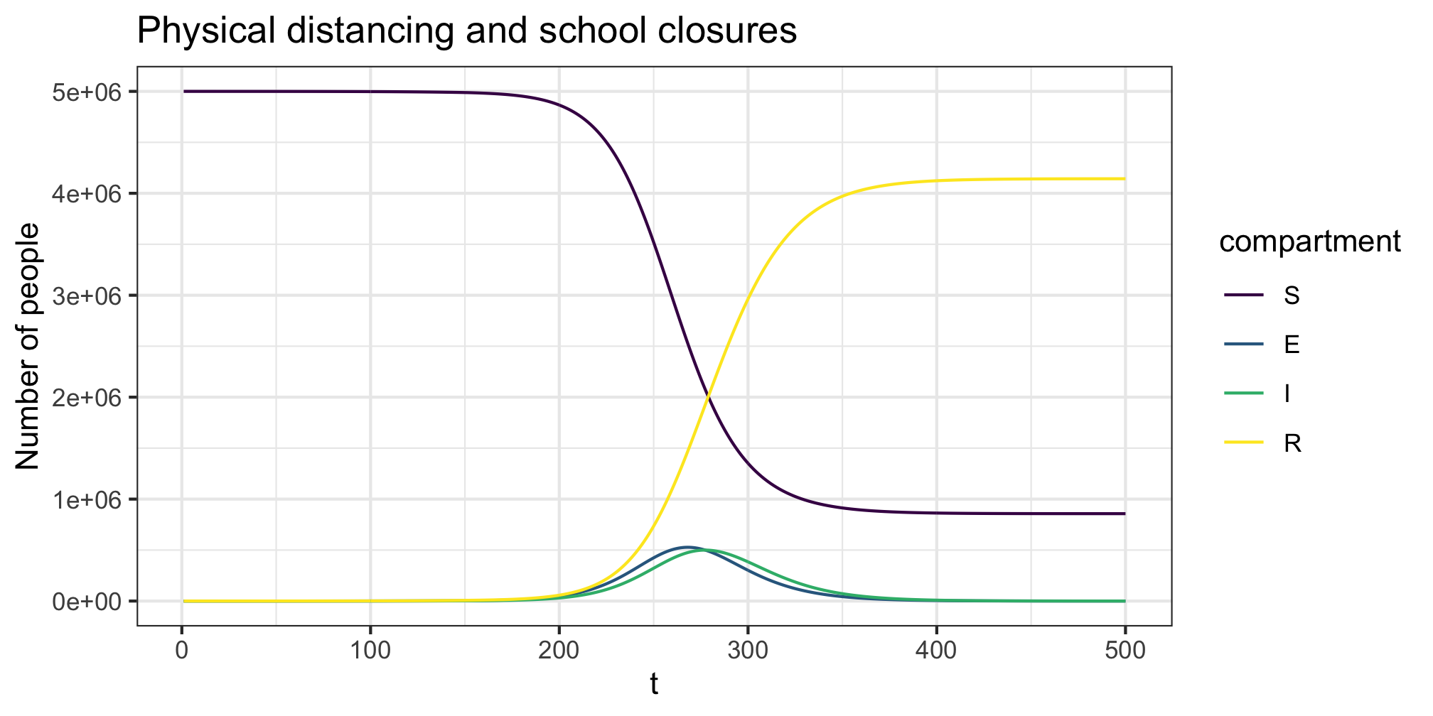
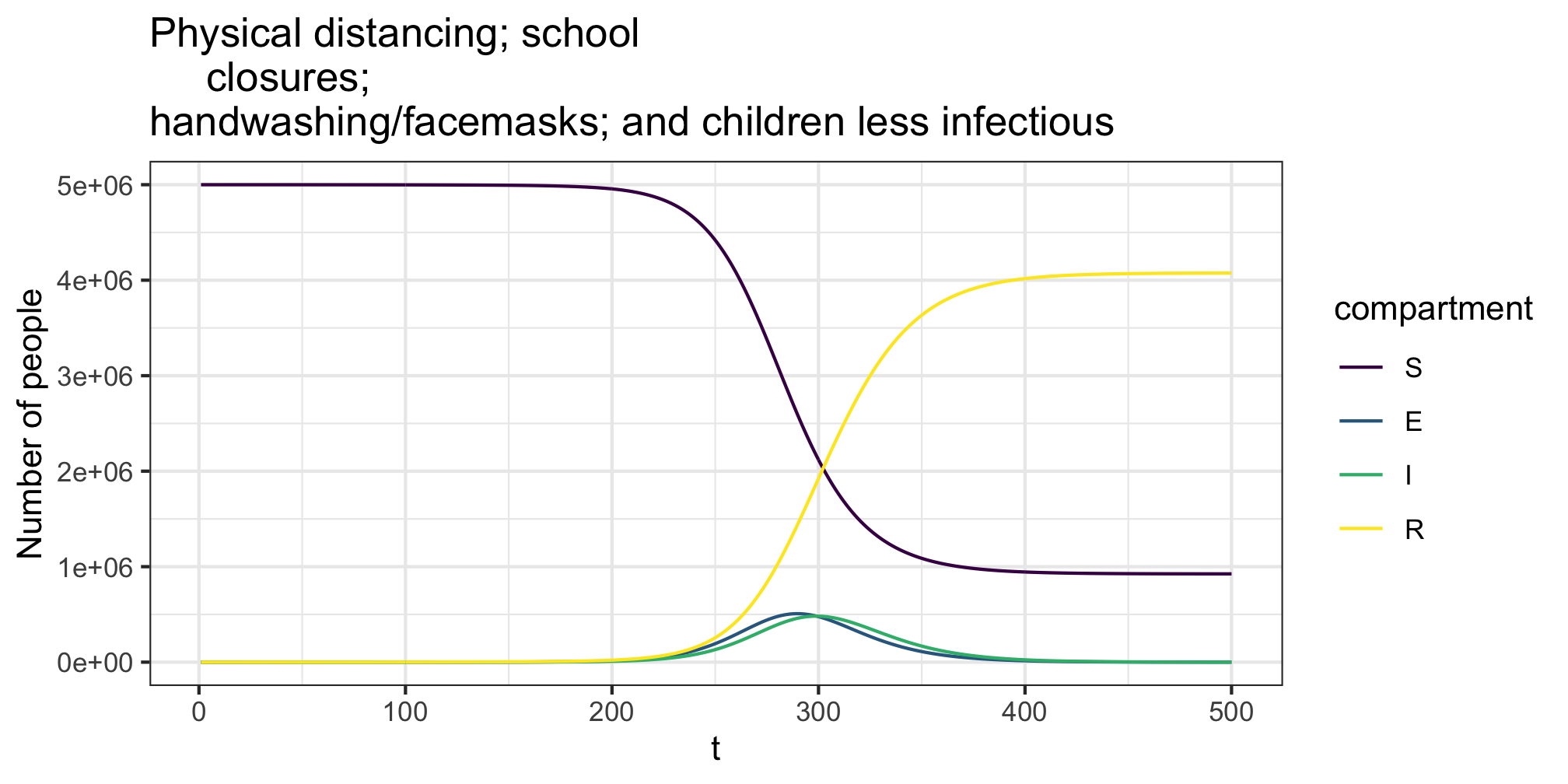
Variation in infectiousness
The im argument to the simulate_*_c function allows us to vary infectiousness and susceptibility across age groups. An entry \(p_{ij}\) of the transmissibility matrix \(im\) denotes the relative chance of an individual in group \(i\) infecting an individual in group \(j\). For example if the average transmission probability is \(p\) the entering \(p_{ij} = 0.8\) indicates an 20% lower change of someone in group \(i\) infecting someone in group \(j\) compared to the average. In the example below we model those under 15 as being less infectious (but as as susceptible). Further using the transmission_intervention we allow for the adoption of general transmission reduction behaviours (e.g. everyone wearing facemasks/hand washing) across the population.
# relative transmissibility matrix
im <- matrix(1,ncol=16,nrow=16)
im[,1:3] <- 0.8
# contact matrices and interventions
cm <- list(all = cm_oz_all, sch = cm_oz_sch)
int_c <- list(sch=contact_intervention(start = 10,stop = 150,reduce = 0.2,
                                      start_delay = 5,stop_delay = 5),
           all=contact_intervention(start = 10,stop = 150,reduce = 0.8,
                                    start_delay = 5,stop_delay = 5))
# transmissibility interventions
int_t <- transmission_intervention(start = 10,stop = 200,reduce = 0.9,
                                  start_delay = 5,stop_delay = 5)
# model and simulation
param <- seir_c_param(R0 = 2.5,gamma = 0.1,sigma=0.1,cm=cm,dist=p_age_oz,
                     contact_intervention = int_c,
                     transmission_intervention = int_t,im = im)
state0 <- seir_c_state0(S = S,E =E,I = I,R = R)
res <- simulate_seir_c(t = 500,state_t0 = state0,param = param)
plot(res,y=c("S","E","I","R"),main="Physical distancing; school
     closures;\nhandwashing/facemasks; and children less infectious")